1.1. Income
Introduction
In the PUMA survey income was included as monthly personal gross income across 15 categories ranging from up to 250€ to more than 6000€.
Frequency personal income
table(WaveOne$SD15_Perseink)
| Response | Frequency |
|---|---|
| don`t know | 39 |
| no answer | 29 |
| up to 250€ | 26 |
| 251 to 500€ | 34 |
| 501 to 750€ | 32 |
| 751 to 1.000€ | 69 |
| 1.001 to 1.300€ | 81 |
| 1.301 to 1.600€ | 68 |
| 1.601 to 1.900€ | 60 |
| 1.901 to 2.200€ | 80 |
| 2.201 to 2.500€ | 112 |
| 2.501 to 3.000€ | 110 |
| 3.001 to 3.500€ | 93 |
| 3.501 to 4.000€ | 64 |
| 4.001 to 5.000€ | 87 |
| 5.001 to 6.000€ | 43 |
| more than 6.000€ | 45 |
Recoding
For the analysis, the scale was recoded into four categories, namely up to 1300€, 1301€ to 2500€, 2501€ to 4000€ and more than 4000€ to provide meaningful categories on sample composition.
In the first step a new variable with missings is defined:
WaveOne$inc <- NA
Recode the lowest five categories capturing all income up to 1.300€ into the new category up to 1.300€:
WaveOne$inc[WaveOne$SD15_Perseink %in%
              levels(WaveOne$SD15_Perseink)[3:7]] <- "up to 1.300€"
Recode the next four categories capturing all income from 1.301 to 2.500€ into the new category 1.301 to 2.500€:
WaveOne$inc[WaveOne$SD15_Perseink %in%
              levels(WaveOne$SD15_Perseink)[8:11]] <- "1.301 to 2.500€"
Contine with the next three categories covering income from 2.501 to 4.000€ into the category 2.501 to 4.000€:
WaveOne$inc[WaveOne$SD15_Perseink %in%
              levels(WaveOne$SD15_Perseink)[12:14]] <- "2.501 to 4.000€"
And summarize the highest income categories from 4.001 to more than 6.000€ into the category more than 4.000€:
WaveOne$inc[WaveOne$SD15_Perseink %in%
              levels(WaveOne$SD15_Perseink)[15:17]] <- "more than 4.000€"
Finally, confirm all Don't know and No answer as missings:
WaveOne$inc[WaveOne$SD15_Perseink %in%
              levels(WaveOne$SD15_Perseink)[1:2]] <- NA # Missings
And format the new variable as factor with specific levels:
WaveOne$inc <- factor(WaveOne$inc,
                      levels = c("up to 1.300€",
                                 "1.301 to 2.500€",
                                 "2.501 to 4.000€",
                                 "more than 4.000€"))
Frequency categorised income
Now take a look at the new variable:
table(WaveOne$inc)
| Response | Frequency |
|---|---|
| up to 1.300€ | 242 |
| 1.301 to 2.500€ | 320 |
| 2.501 to 4.000€ | 267 |
| more than 4.000€ | 175 |
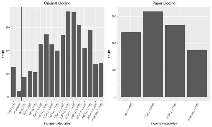
Comparison original vs. paper
The following charts compare the original coding against the coding applied in the article (Table 2, p.11).
p1 <- WaveOne %>%
  # filter all contacted by telephone
  filter(is.na(PUMA1)==FALSE) %>%
  # filter all receiving incentive
  filter(PUMA1==levels(WaveOne$PUMA1)[1] | PUMA1==levels(WaveOne$PUMA1)[2]) %>%
  # filter nonresponse
  filter(valid==1) %>%
  ggplot(aes(SD15_Perseink)) +
  geom_bar(width=0.8) +
  geom_vline(xintercept = 2.5) +
  labs(x="income categories",
       title = "Original Coding") +
  theme(axis.text.x = element_text(angle = 60, hjust = 1),
        plot.title = element_text(hjust = 0.5))

p2 <- WaveOne %>%
  # filter all contacted by telephone
  filter(is.na(PUMA1)==FALSE) %>%
  # filter all receiving incentive
  filter(PUMA1==levels(WaveOne$PUMA1)[1] | PUMA1==levels(WaveOne$PUMA1)[2]) %>%
  # filter nonresponse
  filter(valid==1) %>%
  # drop missings for new income variable
  drop_na(inc) %>%
  ggplot(aes(inc)) +
  geom_bar() +
  labs(x="income categories",
       title = "Paper Coding") +
  theme(axis.text.x = element_text(angle = 60, hjust = 1),
        plot.title = element_text(hjust = 0.5))

grid.arrange(p1,p2, ncol=2)
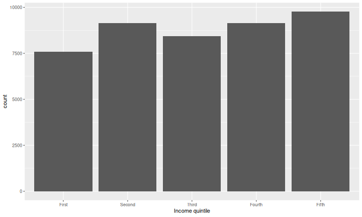
Income quintils
For the nonresponse analysis, the income quintiles from the micro-census data are used.